Mathematica: When the Formula Became the Data

A calculator can tell you what a formula produces once you’ve supplied the numbers. Much mathematical work happens before those numbers arrive.

You might want to rearrange the formula, differentiate it, compare it with another expression, or discover whether two apparently different answers describe the same thing. Assigning a value to every variable would throw away the very relationships you’re trying to study. The computer needs to keep the formula intact long enough to do something useful with it.

Mathematica made that way of working available in an ambitious commercial package. Its first release brought algebra, numerical computation, graphics, and programming together. On the Macintosh, a notebook interface also gave the conversation somewhere to live. A calculation could become part of a document rather than another line disappearing up a terminal window.

The interesting achievement was the coherence. A formula, a list of values, and a graphics description could participate in the same computational language. The software had plenty of individual tricks, but the common machinery made those tricks worth combining.

A system with several authors

Mathematica 1.0 launched on June 23, 1988. Stephen Wolfram’s retrospective places the public presentation at a conference center in Santa Clara, California. The company’s revision history independently records the initial release in June 1988.¹

Symbolic calculation already had a substantial history. Wolfram had used systems including Macsyma and had previously developed SMP, the Symbolic Manipulation Program. Mathematica belongs in that succession of computer algebra systems; calling it the first computer to manipulate algebra would require misplacing several decades.²

Wolfram led the overall design and wrote substantial kernel code. The first edition of Mathematica: A System for Doing Mathematics by Computer names a broader implementation team. Daniel Grayson worked on arithmetic and mathematical algorithms; Roman Maeder handled symbolic integration and polynomial operations; Henry Cejtin worked on central routines. Theodore Gray created front ends, Stephen Omohundro wrote three-dimensional graphics code, David Ballman worked on external interfaces, and Jerry Keiper contributed special functions and numerical operations.³

Those roles help explain the product. It required mathematical expertise, language design, graphics engineering, and an interface capable of presenting the results. None of those jobs becomes optional because the cover has one author’s name.

Stephen Wolfram photographed in 2008.

Stephen Wolfram, July 23, 2008. Later portrait credited to Stephen Wolfram’s PR team/Stephen Faust, source, CC BY-SA 3.0. No alterations.

Keep the symbol

Consider the expression $(x+1)^2$ . A numerical program can evaluate it for a particular $x$ . A symbolic system can retain $x$ as a symbol and change the expression itself.

Mathematica’s first-edition manual documents Expand, which multiplies out products and powers, and Factor, which works in the other direction. These operations let the user choose a representation appropriate to the next task.⁴

Here is a small teaching calculation using functions documented in the 1988 edition. Assume a fresh session in which x has no assigned value:

Expand[(x + 1)^2]
D[(x + 1)^2, x]
Integrate[(x + 1)^2, {x, 0, 1}]
N[7/3]

The corresponding mathematical results are:

Operation	Result
Expand the square	$1+2x+x^2$
Differentiate with respect to $x$	$2+2x$
Integrate from zero to one	$7/3$
Request a numerical approximation	Approximately $2.33333$

These are mathematical results, not a reconstruction of the precise spacing of a 1988 output cell.

The expansion follows ordinary multiplication: $(x+1)(x+1)$ produces $x^2+x+x+1$ , and combining the two middle terms gives $x^2+2x+1$ . Differentiating the expanded polynomial gives $2x+2 $. For the definite integral, an antiderivative is$ x^3/3+x^2+x $. Its value at one is$ 1/3+1+1=7/3$; its value at zero is zero.

The point of the example is the sequence. The result of one operation is still a mathematical object that another operation can use. There is no obligatory stop to transcribe an answer into another application’s idea of what a formula looks like.

The original manual documents D for differentiation and Integrate for both indefinite and definite integration. It also distinguishes exact integer and rational values from approximate numbers written with decimal points.⁵⁶

That distinction is useful even in this tiny calculation. The fraction $7/3$ carries the exact answer. The displayed decimal is a convenient approximation. Keeping the fraction avoids introducing rounding merely because a screen has room for six digits. A decimal point is doing more work here than punctuation usually gets asked to do.

Exactness doesn’t make an input true. If a measurement is only approximate, entering it as a ratio of integers cannot recover information that the instrument never supplied. The representation preserves the claim you gave the computer. You remain responsible for making a sensible claim.

An expression has an inside

Mathematica’s expression model explains why these operations could coexist. The first-edition manual describes expressions with a head and arguments. Familiar operator notation has an underlying functional form: addition uses Plus, multiplication uses Times, and exponentiation uses Power. FullForm exposes that structure.⁷

Conceptually, the square above has this form:

Power[Plus[1, x], 2]

The outer operation is exponentiation. Its first argument is an addition expression, and its second is the exponent two. This is a tree of operations, not a photograph of a printed equation.

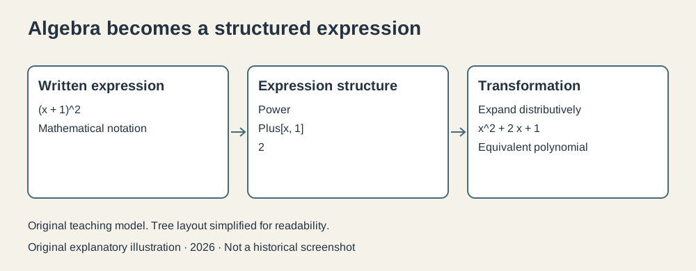
Conceptual expression tree for the square of x plus one.

Original explanatory illustration created in 2026. Argument order in the middle label is conceptual; Mathematica can canonicalize addition order. The image is not a historical screenshot.

A useful analogy is a sentence with grammatical structure. A search through the characters might find an x, but it would not by itself tell you whether that x is a base, an exponent, or one argument among several. The tree records those relationships.

This distinction also separates mathematical transformation from crude text replacement. Replacing every printed x in a document could damage a longer name containing that letter. Operating on a symbol within an expression gives the transformation a more precise target. The software can inspect the parts, recognize a form, and construct a different expression.

Lists fit into this scheme too. A list has a head and a collection of elements; an element may itself be another expression. The same general structural approach can therefore carry a vector of numbers, a nested collection of formulas, or data prepared for a plot. The uniform representation doesn’t mean every operation applies meaningfully to every object. It gives the language a consistent way to describe them.

For the person building a calculation, that consistency reduces the number of separate conventions to remember. For the implementer, it creates opportunities to reuse traversal and transformation machinery. The algebra remains difficult. At least the objects don’t all arrive wearing different identification badges.

A notebook keeps the conversation

Theodore Gray’s account of the front end describes an early aim: a permanent, editable record of interaction with the computational kernel. He chose a vertically scrolling document rather than a fixed two-dimensional drawing surface. A user could insert material into a developing explanation.⁸

The distinction between kernel and front end matters. The kernel performs computation. The front end gives the user a place to enter requests, view results, and organize a document. A useful computational language and a useful document editor are related engineering problems, with quite different failure modes.

A later Wolfram Research account of notebook development dates the original design to 1988 and describes the cell model: headings, narrative, computational input, and results can occupy different cells. Those categories let explanation and execution share a document.⁹

Imagine preparing the polynomial calculation for a student. A text cell explains what $x$ means. An input cell expands the polynomial. Another passage explains the derivative. The numerical answer appears next to the question it answers. The file can preserve the reasoning around the commands, which a bare transcript rarely does elegantly.

This also introduces a responsibility. A document’s visual order and the order in which a person executes its calculations can diverge. Editing an earlier definition doesn’t automatically establish that every displayed result was recomputed afterward. As a general matter, a computational notebook can contain a beautifully arranged account of several different states of an experiment.

A clean session and a deliberate execution order help make that account trustworthy. This is a consequence of combining editable documents with stateful computation, rather than a claim that the first release had a modern notebook auditing feature.

Powerful doesn’t mean unlimited

Mathematica made it easy to request work that was much harder to perform. A short expression can describe an enormous calculation. Expanding a binomial of degree $n$ produces $n+1$ terms; the command grows very little as $n$ grows. Memory requirements feel no obligation to follow its example.

The first-edition discussion of limits emphasizes memory, intermediate expressions, and elapsed time. A compact final answer doesn’t guarantee compact intermediate work. Nor does a convenient command guarantee an efficient solution to every problem.¹⁰

Symbolic integration had mathematical limits as well as practical ones. The original manual gives examples that remain unevaluated when Mathematica cannot express the requested integral in the available standard functions. An unevaluated expression can be an honest answer. It is preferable to a confident formula that happens to differentiate into something else.⁵

The release boundaries deserve care. Version 1.2 arrived in August 1989 with substantial enhancements, including remote-kernel support and rudimentary DSolve capabilities. The revision history places a numerical ordinary differential equation solver and broader symbolic differential equation work in version 2.0, released in 1991.¹¹ Modern Mathematica’s entire mathematical inventory cannot be packed into the 1988 box by writing “and more” after a feature list.

What changed in the work

Mathematica’s lasting contribution is particularly clear in the small example. The user can begin with a formula, change its representation, extract another formula, obtain an exact result, and then request an approximation. The notebook can keep those steps alongside the explanation that makes them useful.

This encourages an exploratory style of work. A person can try a transformation, inspect the result, and revise the next question without building a separate program around every operation. That convenience helps experts experiment and gives learners a way to examine relationships rather than merely watch answers arrive.

It can also make understanding optional for longer than is healthy. A correct derivative doesn’t establish that the original model describes the phenomenon. An attractive plot doesn’t establish that its interesting behavior was sampled adequately. The machine can remove clerical difficulty while leaving intellectual difficulty exactly where it was.

I find that division of labor more interesting than the idea of a computer doing mathematics for us. Mathematica gave formulas a working representation and gave calculations a place in a document. The reader still has to decide what the result means. There is, regrettably, no general command for that.

Stephen Wolfram, “There Was a Time before Mathematica…”, June 6, 2013; Wolfram Research, revision history. ↩
Wolfram, same creator retrospective, discussion of earlier symbolic systems and SMP. ↩
Mathematica: A System for Doing Mathematics by Computer, first edition, 1988, title pages and “About the Developers”, preserved by contributor Stephen Omohundro. ↩
First-edition manual, §1.4.5, “Transforming Algebraic Expressions”. ↩
First-edition manual, §1.5.2, “Differentiation”, and §1.5.3, “Integration”. ↩ ↩²
First-edition manual, §1.1.2, “Exact and Approximate Results”. ↩
First-edition manual, §2.1.1, “Everything Is an Expression”. ↩
Theodore W. Gray, “V3.0: Manifest Destiny”, Mathematica in Education and Research 5(3), 1996; inspected creator’s historical introduction, not used to assign version 3 features to version 1. ↩
John Fultz, “Launching Wolfram Player for iOS”, 2016, historical discussion of the 1988 notebook design. ↩
First-edition manual, §1.4.10, “The Limits of Mathematica”. ↩
Wolfram Research, revision history, entries for versions 1.0, 1.2, and 2.0. ↩