Jupyter: The Calculation Becomes a Document

A chart arrives in an email. Its caption says the new process is better. The reader would like to know which observations were excluded, whether the units changed and what calculation produced the reassuring slope.

A spreadsheet might answer some of those questions. A script might answer others. A notebook offers to put the explanation, executable steps and resulting presentation into the same document.

Project Jupyter was announced at SciPy in 2014 as a home for language-independent tools growing out of IPython. The project’s April 2015 account explains the distinction: an interactive Python environment had accumulated a notebook format, communication protocol, conversion tool and browser application whose usefulness extended beyond Python.¹

That announcement did not invent the notebook in 2014. It recognized that an existing arrangement had become larger than the name of the project carrying it.

To see why this mattered, it is useful to follow a calculation small enough to check without trusting its author.

An analysis with no impressive machinery

Our invented observations are four completion times, in minutes: 10, 12, 14 and 16. We want their mean after applying a fixed two-minute calibration correction to every observation.

The uncorrected total is 52, giving a mean of 13. Subtracting two from every observation produces 8, 10, 12 and 14. Their total is 44, giving a corrected mean of 11.

An explanatory paragraph can state what the correction means. A code cell can define the measurements and correction. Another can perform the calculation. A result can appear immediately below it. The reader need not leave the document to find the prose that interprets the numbers.

For a conceptual three-cell arrangement, write:

# A: inputs
observations = [10, 12, 14, 16]
correction = 2

# B: transformation
corrected = [value - correction for value in observations]

# C: result
mean = sum(corrected) / len(corrected)

The companion check executes these original statements under a modern Python interpreter. It confirms the corrected mean of 11. It is not an execution of IPython 2.0 or evidence about historical notebook performance.

The numbers are deliberately uninteresting. If the mechanism only made sense with a large machine-learning demonstration, it would be harder to distinguish the notebook’s contribution from the calculation’s.

The contribution here is that a computational argument can become inspectable. Inputs, transformation, result and explanation have recognizable places next to one another.

A browser is the desk, not the calculator

The version 2.0 notebook documentation describes code being sent to a kernel associated with the notebook, with returned output displayed below the cell. It distinguishes the browser authoring application from the document itself.²

That separation is easy to overlook because editing, running and reading happen in one visible window. The browser presents the workspace. The kernel holds the running computation’s state. The saved file records document content and outputs.

Those are related things, but they have different lifetimes. Closing a browser window does not necessarily terminate the kernel. The period documentation explicitly describes reconnecting an opened notebook to its still-running session.

In our analysis, the kernel may contain the observation list, the correction and the corrected list. The file may contain code that assigns those names, explanatory text and a displayed mean. The browser may currently be showing an edited cell that has not yet been executed.

All three can look comfortably like one notebook while disagreeing about the latest version of the calculation.

This is not a peculiarity of division or averages. It follows from keeping an interactive session alive while allowing the document that describes it to be edited.

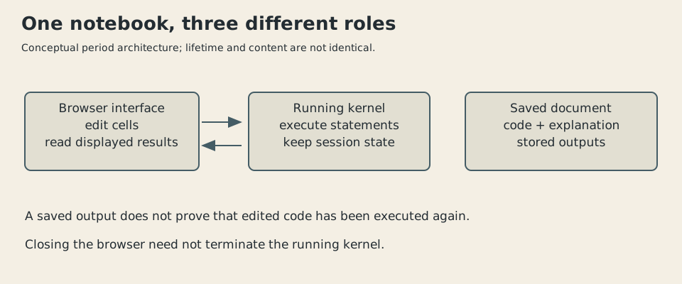
Modern explanatory diagram, drawn in 2026. It illustrates the period notebook arrangement without reconstructing an IPython screen or its messaging implementation.

The page order is not necessarily the execution order

Now change the correction in cell A from two to four. Run A again, then run C without running B.

The observation list remains the same. The correction in the running state is now four. But corrected still contains the list previously calculated using two. C therefore computes 11 again.

The visible inputs now imply a different answer. Running A, B and C in order with the four-minute correction produces 6, 8, 10 and 12, a total of 36 and a mean of nine.

The original check reproduces both sequences: the stale path produces 11; a fresh top-to-bottom execution produces nine. No hidden statistical assumption is involved. One derived value was simply not recalculated.

This is a worked demonstration of stateful execution, not an accusation that the notebook format contains an arithmetic bug. The interactive session did what it was asked to do. The document’s current appearance no longer described the sequence that created its displayed result.

There are good reasons to execute pieces independently. An expensive data-loading step may already be complete. A researcher may want to try a different plot without repeating a long simulation. Interactive exploration is useful precisely because it permits that flexibility.

The cost is that a polished page can conceal an untidy execution history. Moving a cell above another does not undo the order in which their statements ran. Editing a definition does not retroactively recompute values derived from its earlier version.

For this tiny example, a fresh execution of all three cells resolves the mismatch. For a real analysis, that check must also account for external files, library versions, random choices and any work done outside the visible document.

A successful rerun is valuable evidence. It is stronger when the environment and inputs are recorded clearly enough for somebody else to attempt it.

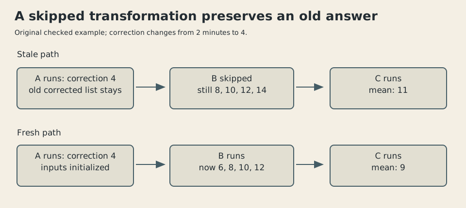
Modern explanatory diagram, drawn in 2026. Both paths were checked with the accompanying Python model; neither is a historical IPython runtime trace.

The file carries a presentation, not a running machine

The period format documentation describes .ipynb files as JSON. Its example uses notebook format version three, including cells, inputs, outputs and a prompt number. Images can be encoded directly in the document.³

That makes a useful package for communication. A reader can inspect saved results without first reproducing the author’s complete environment. An explanation can remain beside a figure rather than becoming a separate file with an uncertain relationship to it.

But the saved mean of 11 in our edited example remains a saved result. It does not prove that the currently visible inputs reproduce 11. The document can preserve a report of an earlier computation even after the code has changed.

The distinction also matters when comparing revisions. Changing one input line is straightforward to understand. Replacing a large encoded image or regenerating many outputs can make the difference between two documents harder to review.

The versioned documentation acknowledges that portability can produce large files and unwieldy differences. A single convenient object is not necessarily the easiest object to audit line by line.

For our miniature calculation, a plain script is sufficient to verify the arithmetic. The notebook’s advantage would be in communicating the reasoning and results together. The script and notebook serve different parts of that work rather than competing to be the only legitimate record.

Readable does not mean re-executed

IPython’s period tools could convert a notebook into static formats, and the documentation describes Notebook Viewer rendering a publicly available document without requiring its reader to install IPython.²

A static page makes the explanation easier to distribute. It also creates a clear boundary: reading the displayed calculation is different from running it.

Our report might explain why a calibration correction was appropriate and show the resulting nine-minute mean. A static reader can check the argument’s structure and perhaps the small arithmetic. They have not thereby checked that the original data file was correct or that a larger calculation ran under the claimed dependencies.

Nor does exporting to a different format manufacture missing context. If the correction’s units or justification were omitted from the notebook, a beautifully rendered PDF would preserve the omission with better typography.

The notebook makes room for an explanation. Its author still has to write one.

The project separated things that had different jobs

IPython 2.0, released in April 2014, added a modal notebook interface, directory navigation, interactive widgets and a notebook security model. Its release notes identify these as period developments.⁴ They should not be mistaken for later JupyterLab features.

The 2015 split account, meanwhile, explains that the notebook format, protocol and experimental tools needed different release schedules. Giving the language-independent parts their own packages allowed those boundaries to become organizational as well as technical.

That is a more consequential interpretation of Jupyter’s 2014 arrival than a story about merely changing a logo. The project distinguished a language’s interactive environment from the broader machinery for communicating computational work.

It did not make every notebook language-independent internally. Our original example remains Python code. A suitable kernel and the required environment are still necessary to execute it. The generality belongs to the surrounding arrangement and interfaces, not to a promise that arbitrary code will run everywhere.

The resulting document can be unusually hospitable to a reader. Here are the observations. Here is the correction. Here is the calculation. Here is what the author thinks it means.

It can also be unusually persuasive when one of those parts is stale. Jupyter helped make the calculation into a document. A careful author must still make the document an honest account of the calculation.

Sources

Footnotes

1. Project Jupyter, “The Big Split”, April 16, 2015, announcement history and package separation. Official about page corroborates 2014 origins. ↩

2. IPython, release 2.0.0 notebook documentation, introduction, opening notebooks, code cells and workflow sections inspected. Some shortcut documentation was already stale; no exact shortcut claims rely on it. ↩ ↩²

3. IPython, release 2.0.0 conversion and JSON documentation, inspected in full. Format-three example is period-specific, not a description of today’s file schema. ↩

4. IPython, 2.x release notes, 2.0 section, April 2014 features. Preserved maintained documentation includes later 2.x releases. ↩