MATLAB: Giving the Matrix a Command Prompt

A student wants to solve a system of equations. The numerical library has an excellent routine for doing so. Between the student and the routine sits a modest obstacle course: write a Fortran program, prepare the data, arrange the call correctly, compile, run, and inspect the result. Then discover that one number was wrong and repeat the ceremony.

Cleve Moler’s early MATLAB shortened that journey. It provided interactive access to numerical linear algebra, making a matrix something you could enter and manipulate directly. The abbreviation stood for Matrix Laboratory. It was an apt name: you could try something, inspect it, and change the experiment while the problem was still fresh in your head.

The version that became a commercial product in 1984 was a further development, not MATLAB’s first existence. Keeping those stages separate makes the story more interesting. The original solved an educational access problem. The commercial product turned that access into a broader working environment for engineers.¹

The mathematics came first

MATLAB’s early capabilities drew on LINPACK and EISPACK, numerical software libraries concerned with linear systems and eigenvalue problems. Moler participated in that numerical computing community and wrote the original interactive calculator in Fortran. It let students use the mathematical routines without making Fortran programming the admission requirement.¹

This is an unusually clear example of software putting an interface around substantial prior work. The reliable algorithms mattered. The new access pattern mattered too. A powerful routine that is awkward to reach can be less useful in practice than its mathematical sophistication suggests.

Jack Little recognized a commercial opportunity, and Little and Steve Bangert developed a new implementation in C for personal computers. Moler, Little, and Bangert founded MathWorks in 1984. PC-MATLAB added a programming environment and graphics to a system whose academic ancestor had been much more narrowly a matrix calculator.²

Moler’s retrospective timeline places PC-MATLAB, graphics, and FFT capability in 1984, the Control System Toolbox in 1985, and the Signal Processing Toolbox in 1987. It places sparse matrices in 1992 and the integrated desktop in 2000. The modern MATLAB window, with its coordinated panels and editors, would therefore make a misleading illustration of the original commercial milestone.¹

The historically important interface was an interactive conversation with numerical objects. An engineer could move between a calculation and its visual interpretation without turning every small experiment into a separate software project. That is an excellent place to spend a computer’s patience.

What a matrix buys you

A matrix is a rectangular array of values. Its importance isn’t simply that it stores numbers tidily. Many scientific problems can be expressed as operations on entire arrays, with well-understood relationships between their dimensions.

Consider a deliberately small teaching problem. A workshop makes two products, represented by unknown quantities $x$ and $y$. Each unit of the first product uses two units of material A and one unit of material B. Each unit of the second uses one unit of A and three units of B. Available totals are eight units of A and nine units of B.

The equations are

$$2x+y=8,\qquad x+3y=9.$$

In matrix form,

$$A\mathbf{q}=\mathbf{b},\qquad A=\begin{bmatrix}2&1\\1&3\end{bmatrix},\quad \mathbf{q}=\begin{bmatrix}x\\y\end{bmatrix},\quad \mathbf{b}=\begin{bmatrix}8\\9\end{bmatrix}.$$

The rows correspond to constraints; the columns correspond to the unknown quantities. That orientation matters. A matrix containing the same four coefficients in the wrong places represents a different problem. Rectangular tidiness is not mathematical correctness.

An illustrative MATLAB session uses the longstanding matrix and backslash notation:

A = [2 1; 1 3];
b = [8; 9];
q = A\b

The result is $x=3$ and $y=2$. Substitution verifies it: $2(3)+2=8$ and $3+3(2)=9$. These are invented data, and the syntax example explains the matrix model rather than reproducing a session from a surviving 1984 executable.

Semicolons within the brackets separate rows. A space separates entries on the same row. A semicolon after an assignment suppresses its ordinary displayed result, so a sequence can avoid announcing every intermediate matrix like an overenthusiastic clerk.

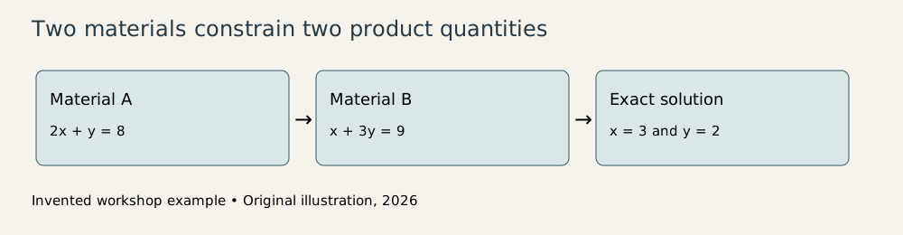
Original explanatory diagram, 2026; invented workshop example, not historical MATLAB output.

The backslash is a decision about algorithms

The expression A\b asks for a solution to the linear system. It does not ask the user to write out all the steps of elimination. This is a useful distinction between stating a numerical task and implementing its algorithm.

For our two-by-two example, ordinary algebra is enough. Multiply the second equation by two and subtract the first: $5y=10$, so$y=2$. Substitute into the first equation to find$x=3$. With hundreds of unknowns, manually extending that calculation becomes tedious. A numerical routine organizes the work, handles representation, and chooses the appropriate steps for its supported case.

It is tempting to describe solving as “invert A and multiply.” The mathematical relationship can be useful on paper, but explicitly computing an inverse generally performs unnecessary work when the real task is one solution vector. The better interface lets the user state the desired solution directly.

There are still assumptions. Some systems have no unique solution. Others respond dramatically to small changes in the input. Numerical linear algebra has to consider the properties of the system and the limitations of floating-point arithmetic. Making the command short doesn’t make the underlying mathematics optional.

One important practical check is the residual, $A\mathbf{q}-\mathbf{b}$. For our exact small solution, it is the zero vector. In a numerical calculation it may contain tiny nonzero entries caused by rounding. A small residual says the calculated result nearly satisfies the supplied equations; it doesn’t, by itself, guarantee the supplied equations accurately model the workshop.

That separation is central to useful technical computing. Algorithm quality, numerical conditioning, and model quality are different concerns. MATLAB made trying the computation convenient. The scientist or engineer still had to decide what the computation meant.

Almost the same equations can be a different problem

Here is another teaching system:

$$x+y=2,\qquad x+1.0001y=2.0001.$$

Its exact solution is $x=1$, $y=1$. Change only the second right-hand side to 2.0002 and the exact solution becomes $x=0$, $y=2$. A change of 0.0001 in one supplied total has produced a large change in the solution.

The reason becomes visible on subtraction. The two equations are nearly the same. Their difference says $0.0001y=0.0001 in the first case and \0.0001y=0.0002$ in the second. The small distinguishing information bears a great deal of responsibility.

This example illustrates conditioning: sensitivity of the mathematical answer to input changes. It isn’t a bug in an interpreter or evidence that matrices are temperamental. An accurate program can faithfully calculate an answer that is highly sensitive because the problem itself is highly sensitive.

An interactive environment is valuable here because it supports experiments with perturbations. Change a measurement, solve again, compare results, and inspect whether conclusions remain stable. That is a substantive part of analysis rather than a decorative demonstration after the “real” calculation.

The same approach applies to fitting data. A line fitted to noisy observations can give useful estimates, but its meaning depends on the observations, the assumed model, and the spread of the data. A confident-looking plot can still represent an underdetermined argument. The graphics have excellent manners; they don’t cross-examine the author.

From calculator to working environment

The commercial system’s broader programming facilities allowed calculations to be organized and reused. Graphics gave a way to inspect relationships that a printed column of numbers might conceal. Toolboxes could extend the environment toward particular technical fields. Each addition reinforced the original idea: keep mathematical operations near the person experimenting with the problem.¹

That convenience carries tradeoffs. An interactive session can accumulate state. A result may depend on a variable defined much earlier, or on a changed input whose provenance isn’t obvious. Saving a reproducible program becomes important when an exploratory calculation starts supporting a report or design decision.

Arrays also use memory. A representation that is natural mathematically may be expensive computationally. The early commercial milestone shouldn’t be credited with later sparse representations simply because modern MATLAB handles them well. Improvements in the environment changed the feasible size and variety of its problems over time.

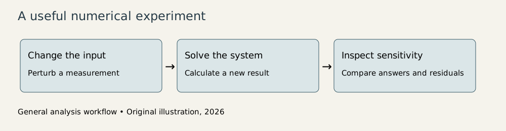
Original explanatory workflow, 2026; a general numerical experiment, not a historical interface reconstruction.

I find MATLAB’s original choice more enduring than any particular collection of toolboxes. It made the matrix the ordinary object of interaction. That put a rich body of numerical methods behind expressions a technical user could read, try, and revise.

The program’s success didn’t require replacing numerical expertise with a friendlier prompt. It allowed that expertise to be used more directly. The student or engineer could spend more attention on choosing the equations, checking their sensitivity, and understanding the result. Those were always the difficult parts. MATLAB made more of the surrounding ceremony willing to get out of the way.

Footnotes

1. Cleve Moler, A Brief History of MATLAB, creator’s retrospective on the Fortran calculator and version milestones. Historical details from this source are kept compact; examples here are original explanations. ↩ ↩² ↩³ ↩⁴

2. Cleve Moler oral history, interviewed by Thomas Haigh, March 8–9, 2004, development and commercialization with Little and Bangert. SIAM interview record. ↩