CTSS: Save Your Place, Let Somebody Else Work

A programmer needs to try a small correction. Another program is already running a long calculation. The correction may require very little computing, but that fact is unhelpful if it has to wait behind the entire calculation.

Time sharing changes the arrangement. Give programs limited turns, preserve their progress between turns and let an interactive user make another request without owning the whole machine.

The processor hasn’t become several processors. The operating system has become responsible for making short pieces of several people’s work fit around one another.

CTSS, the Compatible Time-Sharing System, was an early practical exploration of that responsibility. Its attraction was easier interaction; its engineering depended on keeping the interrupted work intact.

An experimental beginning

The original programmer’s guide dates an experimental early CTSS demonstration at MIT to November 1961.¹ The 1962 paper by Fernando Corbató, Marjorie Merwin-Daggett and Robert Daley describes the system, originally written for the IBM 709 and converted to the 7090.²

That account has three interactive typewriters and a background user. The initial organization keeps one user program in core at a time, with the supervisor retained separately and magnetic tape used for swapping and private files. Protection, relocation and I/O trapping are part of the modified 7090 environment.²

These are early boundaries. Later CTSS hardware and disk services aren’t being inserted into the 1961 demonstration. The article’s schedules use invented work units, rather than presenting a paper’s analytical timing assumptions as a measured initial quantum.

A working experiment is already worth understanding without turning it into every later feature of the service.

Two jobs, eight units of work

For an original teaching schedule, suppose job A needs six units of processor work and job B needs two. Both are ready at time zero. One unit is a chosen model interval, not a second of CTSS execution.

First run A until it finishes, then B. A occupies time 0 through 6. B gets time 6 through 8. B’s short calculation finishes at time 8.

Now give each ready job a turn of one unit. This maximum turn length is called a quantum. Alternate while both jobs still need work:

Interval:  0–1  1–2  2–3  3–4  4–5  5–6  6–7  7–8
Job:        A    B    A    B    A    A    A    A

At time 4, B has received its two units and is finished. A has received only two of its six, so it continues for another four.

The total useful processor work is still eight units. B’s completion moved from time 8 to time 4 because the order changed. We haven’t claimed that sharing manufactured additional arithmetic capacity.

For a person awaiting B’s answer, the difference is concrete. The small task can finish before the large task is complete.

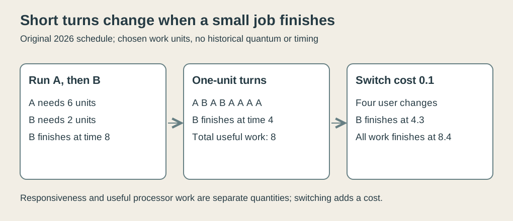Original explanatory SVG, created in 2026. Jobs, interval lengths and switch costs are invented teaching values, not a CTSS benchmark.

Save more than the name

Stopping A isn’t enough. The system has to preserve what A needs in order to continue: the place in its computation, its working values and the relevant stored contents.

Our model makes that responsibility small enough to inspect. A performs six steps, incrementing its counter by one each time. B performs two steps, incrementing its own counter by ten.

After A’s first turn, its saved state is position 1, counter 1. B’s first turn produces position 1, counter 10. A’s next turn must restore A’s state, producing position 2, counter 2.

If A instead receives B’s counter, its next result becomes 11. If its state is reset to zero every turn, repeated execution of the first step never becomes six completed steps.

Neither failure is a scheduling preference. Both violate the meaning of “resume.”

The program’s next position and its counter belong together. Restoring only one can combine a later instruction with an earlier value, or repeat a completed instruction using a later value. A saved-state record is a set of relationships, not a bag of numbers that can be selected independently.

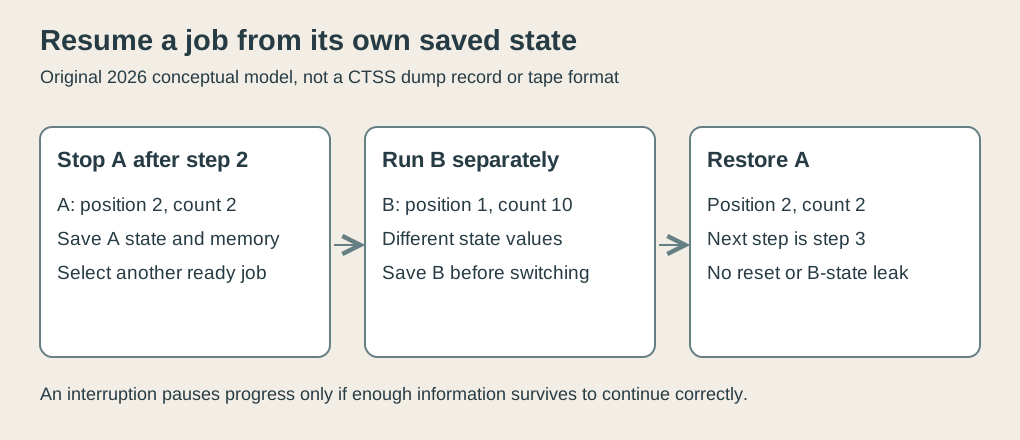Original explanatory SVG, created in 2026. Position/counter pairs are chosen model state, not actual CTSS register or tape-dump layouts.

Our checker verifies that both jobs retain separate state and finish with A’s counter at 6 and B’s at 20. It also records the resumed positions to ensure the steps weren’t simply counted in a final total after being restarted incorrectly.

Actual operating systems preserve much more than two fields. The model explains the obligation without claiming to recreate an old machine’s full register set or memory-transfer procedure.

Shared residency needs boundaries

Early CTSS’s one-user-in-core arrangement and tape swaps make the storage aspect visible.² To run another user in the same working region, the previous contents must survive elsewhere if they are to be restored later.

The schedule therefore depends on a distinction between a job’s logical state and where that state is currently resident. A program can still exist while it isn’t the program presently using the processor or occupying the user working region.

The supervisor has different responsibilities. It chooses work, handles transitions and keeps the records needed to recover each user. If an ordinary program can casually overwrite those records, its arithmetic mistake can become everyone else’s scheduling mistake.

Protection and mediated access help establish that boundary. They don’t make a shared machine infinitely reliable. The scheduling software and its saved data are themselves part of the system that must work correctly.

For our original model, the supervisor owns a dictionary of per-job records. The current job gets only its restored position and counter. This is a conceptual organization, not an assertion about CTSS’s internal data structures.

Switching consumes time

The eight-unit schedule ignored the cost of changing jobs. Add a hypothetical 0.1 unit for each change from one user to the other. Count neither the initial dispatch nor a final transition out of the model.

The one-unit sequence has four changes: A to B, B to A, A to B, then B to A. Once B finishes, the remaining A turns need no change of user.

The total becomes $8 + 4 \times 0.1 = 8.4$. B finishes after four units of useful work and three prior changes, at time 4.3.

Increase the quantum to two useful units. The sequence is A for two, B for two, then A for its remaining four. There are two changes. Total elapsed time becomes 8.2, and B completes at 4.1.

In this particular workload, the larger quantum produces both lower overhead and a slightly earlier B completion. That doesn’t establish a universal optimum. B’s first opportunity to execute begins later: after two A units rather than one.

A still longer first A turn of six units delays B’s first work until 6.1 and completion until 8.1. The overhead is lower again, but the interactive opportunity is worse.

The chosen values make a tradeoff inspectable. Real turn lengths and swap costs depend on the system and workload. These numbers aren’t evidence for an original CTSS performance claim.

Waiting isn’t running slowly

Add another original example. Job C computes for one unit, then waits for input until time 5, then needs one final unit. Job D needs three units of computation and is ready immediately.

Run C from time 0 to 1. While C waits, run D from 1 to 4. At 4, neither has ready work: D is complete and C’s input hasn’t arrived. The processor can be idle until 5, when C becomes ready and finishes at 6.

C’s elapsed duration is six units. Its useful processor work is only two.

Charging it six units of computation would confuse waiting with execution. Repeatedly giving the waiting job empty turns would also waste opportunities to run D. A scheduler needs a notion of readiness, separate from whether a job has finished.

The CTSS paper explicitly describes an I/O-wait status and return to working status.² Our timeline uses invented readiness times to illustrate that distinction without reproducing the actual buffer rules.

A user pausing to think is another reason an interactive session needn’t consume its maximum possible processor share continuously. There is useful room between “the session exists” and “the program has work the processor can perform now.”

Several measures of a good schedule

B’s example gives at least three measurements: time before its first turn, time before its completion, and total time until both jobs finish. They answer different questions.

A person typing a small command may care most about prompt first response. A long-running calculation may care about overall completion. The installation also has to account for time spent changing state rather than computing.

Our checker preserves those distinctions. It tests useful work totals, per-job completion and the chosen overhead separately. It then checks the C/D readiness timeline and verifies that waiting time didn’t become fictitious computation.

The implementation uses modern Python. It doesn’t run CTSS, a 709/7090 simulator or the historical tape-swapping machinery. Its result is a verified example of a defined policy, not evidence that the original service executed these exact schedules.

Keep the unfinished work intact

I find saved state the most important detail in the story. Interleaving makes a schedule look fair only if each program receives back the computation it left behind.

CTSS made interactive sharing a system problem: preserve progress, separate users, recognize waiting and choose another ready task. Our two-job examples show why neither the fairness nor the speed can be summarized by one turn length.

The shared computer can give somebody else a turn. The useful promise is that, when yours returns, it still knows where you were.

Footnotes

1. CTSS Programmer’s Guide, original preface, page vi, dating the early demonstration to November 1961. ↩

2. Fernando J. Corbató, Marjorie Merwin-Daggett and Robert C. Daley, “An Experimental Time-Sharing System”, 1962, pages 335–344. Early configuration and operating queues are distinguished from later service and analytical proposals. All numerical schedules and two-field state examples here are original teaching models. ↩ ↩² ↩³ ↩⁴