TensorFlow: Give the Calculation a Graph

A short program can look as though it is multiplying two values while actually constructing an instruction to multiply them later.

That distinction was central to the first public TensorFlow. In its early Python interface, developers assembled a graph of operations, then asked a session to execute the part needed for a result. The graph was a description with a life separate from any one execution.

Google announced the open-source release on November 9, 2015. Jeff Dean and Rajat Monga described a successor to the internal DistBelief system, intended to be more flexible and easier to share outside Google’s infrastructure.¹

This article follows the public version 0.5.0 documentation. It does not put today’s TensorFlow execution habits into a 2015 example or treat the launch’s performance claims as measurements made here.

A very small model is enough to explain the machinery. It also makes it harder for the impressive word learning to conceal ordinary arithmetic.

A prediction with two adjustable numbers

Consider a fictional prediction rule:

prediction = weight × input + bias

Use input two and desired output six. Start with weight one and bias zero. The rule predicts two, missing the target by negative four.

Define loss as the square of that difference. Negative four squared gives 16. The square gives us a nonnegative measure, with zero when this prediction agrees exactly with this target.

Nothing has been learned yet. We have specified a rule, chosen initial parameters and defined a way to measure its error.

A graph can represent those relationships. A multiplication takes weight and input. An addition combines its result with bias. A subtraction compares the prediction with the target. A square produces the loss.

The arrows matter because each operation requires the results of its predecessors. If the requested output is loss, the system needs the upstream prediction. A node’s visible position in a diagram is less important than its dependencies.

In a bigger model, this description can become much more elaborate. The small example retains the same distinction between data, parameters and operations without requiring a reader to accept a complicated network on faith.

Construction is not execution

The version 0.5.0 basic-usage document explicitly separates a construction phase from a session-based execution phase. It defines operations as graph nodes and tensors as typed multidimensional arrays passed between them.²

A Python object returned while constructing an operation can stand for its eventual output. It is not necessarily holding the calculated value already. The period FAQ explains this point using matrix multiplication.³

For our example, constructing the loss graph describes how loss depends on input, weight, bias and target. Requesting the loss in a session is the step that performs the required calculation.

That separation can be surprising to a programmer accustomed to each statement performing its visible arithmetic immediately. It is also useful. A description of the whole computation gives the execution machinery more information about dependencies and opportunities to place work on available devices.

The document describes CPUs and GPUs as execution devices. That does not mean our tiny multiplication automatically benefits from being sent to a GPU. Managing work has costs, and the example is far too small to justify a hardware performance conclusion.

The companion arithmetic check uses plain modern Python. It verifies the numbers and derivative relationships. It does not construct a TensorFlow graph, start a TensorFlow session or measure device placement.

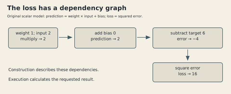
Modern explanatory diagram, drawn in 2026. This is a locally authored graph of the original arithmetic example, not a 2015 TensorBoard capture.

The gradient gives a direction, not a finished answer

To adjust the parameters, ask how the loss changes when each parameter changes a little.

Let the error be prediction minus target. For this rule, the derivative of squared loss with respect to weight is twice the error times input. The derivative with respect to bias is twice the error.

At the starting values, error is negative four and input is two. The weight derivative is negative sixteen. The bias derivative is negative eight.

Choose a learning rate of 0.05 and subtract that rate times each derivative from its parameter. Weight becomes 1.8; bias becomes 0.4. The new prediction is four. Error is negative two and loss is four.

The first update has reduced loss from 16 to four. A second update gives weight 2.2 and bias 0.6. Prediction becomes five and loss becomes one.

The companion script checks those values using exact rational arithmetic. It also checks the analytical derivatives against a small central difference of the loss function. That is a check of this original example, not a test of TensorFlow’s automatic differentiation.

The version 0.5.0 introductory tutorial supplies period evidence for the larger arrangement: a loss expression, GradientDescentOptimizer, an operation produced by minimize, initialization and repeated session execution.⁴ Its own example fits a plane to invented data; the scalar example here is independently constructed.

TensorFlow’s contribution was not to invent gradient descent. It placed differentiation and parameter updates within the same computational system used to describe the model.

A developer could specify the loss rather than manually derive every update for every large model. That convenience remained dependent on the supported operations and the actual graph being constructed correctly.

The size of the step is a decision

The negative gradient tells us a direction of local decrease. It does not authorize an arbitrarily large movement.

Use a rate of 0.5 instead of 0.05 for the first update. Weight becomes nine and bias becomes four. With input two, prediction becomes 22. The error is sixteen and the loss is 256.

Our supposedly helpful update has made the starting loss of 16 much worse. The check confirms this result too.

The arithmetic is a useful antidote to a vague account in which an optimizer simply improves a model. An optimizer follows an algorithm with chosen parameters. Its behavior depends on the objective, scale and inputs supplied to it.

A declining training loss also answers a narrow question. With just one observation, many combinations of weight and bias can predict six from input two. The example cannot establish which rule would perform well on input values it has never seen.

Weight three and bias zero work for this observation. Weight two and bias two also work. They disagree elsewhere. A perfect fit to one target is not enough information to choose between them.

Neither TensorFlow nor any other execution system can extract missing evidence from a loss definition. The developer still needs appropriate data and a meaningful evaluation of what the model is supposed to do.

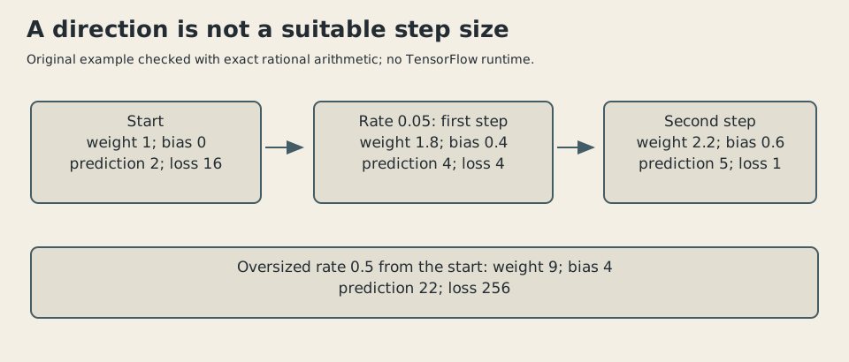
Modern original arithmetic illustration, drawn in 2026. Values were checked with rational arithmetic; they are not TensorFlow timings or measured model accuracy.

Variables preserve what training changes

A graph describing a rule and the current values of its parameters are different parts of a model. Training repeatedly uses the rule while changing those parameter values.

The period documentation describes Variables maintaining state across executions. Their initialization and assignment are themselves operations that must be run.²

For our example, the graph’s multiplication does not need to be reinvented after every step. The weight and bias change. Running the relevant operations again uses the updated values.

Inputs can also vary between executions. The early interface’s feed mechanism permits runtime values to be supplied, commonly through placeholders. The graph can then describe a recurring calculation while each run receives a particular set of data.

That is useful for repeated training or inference. It also introduces distinctions a developer has to understand: the definition, initialized state, supplied input and requested output.

An instruction to assign a parameter is not the completed assignment until its execution occurs. A graph that has been assembled is not a trained model merely because it contains an optimizer.

The period basic-usage file contains inconsistent variable names in one counter example. The article does not copy that snippet or claim to have run it successfully. Reading a historical tutorial and testing a historical program are separate activities.

Public scope matters more than internal scale

Google’s launch story naturally drew on substantial internal machine-learning work. The public FAQ supplies a narrower boundary: the initial open-source release supported multiple CPUs and GPUs in one computer, while a distributed version was still being developed.³

It would therefore be misleading to make the 2015 public download inherit every distributed capability suggested by Google’s internal experience. The intended architecture and the released package are related, but they are not the same artifact.

The launch’s open licensing and associated tools made computational ideas easier to exchange as software. The graph was a common object around which model authors, execution machinery and inspection tools could organize their work.

That did not remove the surrounding decisions. A useful model still needed suitable inputs, a defensible objective, compatible operations and an evaluation beyond the examples used for training. Hardware capability did not repair a bad loss function.

TensorFlow’s first public year is consequently most instructive as an effort to make the calculation explicit and reusable. Construct a graph. Initialize what has state. Supply inputs. Request the work. Adjust the parameters according to a defined rule.

The prediction may still be wrong. At least the route from two to that wrong answer has become something the program can describe—and something a careful reader can inspect.

Sources

Footnotes

1. Jeff Dean and Rajat Monga, TensorFlow open-source announcement, November 9, 2015. Launch purpose and Apache 2.0 release; benchmark rhetoric not adopted. ↩

2. TensorFlow, 0.5.0 basic usage, inspected in full. Graph/session distinction, tensors, variables and feeds; inconsistent counter snippet not executed. ↩ ↩²

3. TensorFlow, 0.5.0 FAQ, opening through graph, sessions, release distribution limits, variables, shapes and TensorBoard sections inspected. ↩ ↩²

4. TensorFlow, 0.5.0 introduction, inspected in full. Period gradient-descent training arrangement, not the article’s original scalar calculation. ↩