Photoshop 1.0: The Photograph Became a Set of Numbers

A photograph on paper is an object. A photograph inside an image editor is a collection of measurements arranged in a grid. That change of representation creates an extraordinary amount of freedom. It also makes “make it a little sharper” a much more complicated instruction than it sounds.

The software can change a value, move a region, or apply the same transformation to thousands of samples. It has no automatic understanding of which changes improve the image. A face, a cloud, and a scanner defect can all arrive as numbers with excellent administrative consistency.

Photoshop’s first commercial release put a broad set of these operations into one Macintosh application. It helped connect scanning, image manipulation, and publishing preparation. The interesting engineering wasn’t simply that pictures could be altered. It was that the picture had a representation on which many different tools could work.

An application grew out of utilities

Adobe dates Photoshop’s retail debut to February 19, 1990. The Computer History Museum records an earlier path: Thomas Knoll wrote an image-display program in 1987, the brothers developed it toward a commercial product in 1988, and Adobe agreed to distribute an enhanced version in April 1989.¹²

Thomas was studying computer vision at the University of Michigan. John Knoll worked at Industrial Light & Magic, where digital image processing was becoming relevant to visual effects. Thomas’s later interview describes John asking for separate image utilities to be gathered into one application. John also contributed plug-ins while Thomas built the base application.¹

That request is a useful explanation of what an application adds. Several capable tools can still require awkward handoffs. A shared document, consistent selection, and common interface let the user combine operations without continually transporting the image between programs.

The early program had already reached a small audience before Adobe’s release. Barneyscan bundled roughly two hundred copies of version 0.87 with scanners. That earlier distribution is distinct from Photoshop 1.0’s 1990 launch.²

The preserved first-generation source is version 1.0.1, written primarily in Pascal with Motorola 68000 assembly where useful. It is available through the museum under restricted noncommercial terms. Its historical accessibility does not make it freely redistributable open-source software.²

The application was substantial, but it wasn’t the modern product squeezed onto a few old disks. Most conspicuously, the compositing layers now associated with Photoshop arrived with version 3 in 1994.² Understanding version 1 begins by putting that later convenience aside.

An image has dimensions twice

A sampled image has a width and height in pixels. A printed image has a width and height in physical units. A resolution setting connects them.

The original 1990 guide explicitly distinguishes image resolution, measured in pixels per inch, from an output device’s resolution in dots per inch. These quantities describe different parts of the process.³

Consider an invented RGB image measuring 1,200 pixels across and 800 pixels down. It contains:

$1200\times800=960{,}000\text{ pixels}.$

If each pixel has one eight-bit sample for each of red, green, and blue, its raw channel samples occupy:

$960{,}000\times3=2{,}880{,}000\text{ bytes}.$

That is the sample data in our model, excluding file headers, compression, saved selections, and the editor’s working storage. It isn’t a prediction of the application’s complete memory use.

At 300 pixels per inch, the printed width is $1200/300=4$ inches. The height is $800/300=2\frac23$ inches. Change the print interpretation to 150 pixels per inch while retaining the same samples, and the width becomes eight inches, with a height of $5\frac13$ inches.

The image has become physically larger without acquiring any new measurements. Each inch now contains fewer of the existing samples.

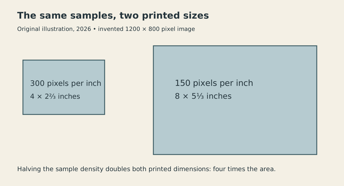
Original explanatory illustration, 2026. Invented image and print dimensions; rectangles show the 1:2 ratio of both printed dimensions. Not a Photoshop screenshot.

This is why a resolution number can be misleading when detached from pixel dimensions. “Three hundred pixels per inch” says how densely samples are distributed at a chosen size. It doesn’t by itself tell you how many samples exist. A very small image can have an impressive-looking setting and still be a very small image.

Nor does a printer capable of placing many dots per inch require one independently supplied image pixel for each dot. Printing has its own machinery for representing tones. The editor’s grid and the printer’s marks are connected, but they aren’t identical grids by definition.

Resampling is a different operation

The first guide describes a Page Setup sizing option that changes output size without changing the pixel count. It separately describes a Resample command that changes the image’s samples. The distinction was already part of the original product.⁴

Suppose we want the same eight-inch width at 300 pixels per inch. We now require 2,400 pixels across. Keeping the aspect ratio requires 1,600 pixels down. Our raw three-channel model grows to:

$2400\times1600\times3=11{,}520{,}000\text{ bytes}.$

Doubling both dimensions quadruples the pixel count. An image can make an apparently modest request of the interface and a rather immodest request of memory.

The new pixels must get values from somewhere. Interpolation estimates them from available samples. It can produce a useful enlarged representation, but it hasn’t discovered detail that the scanner failed to record.

Downsampling presents the opposite problem. Reducing both dimensions by half leaves one-quarter as many pixels. The program has to summarize information in fewer locations. Some detail is lost. Enlarging that reduced result afterward doesn’t restore the discarded measurements.

A simple one-dimensional example makes the issue visible. Imagine two neighboring grayscale samples, 0 and 255. Combining them by an ordinary arithmetic average gives 127.5, a middle value. A sharp black–white boundary has become one summary sample. This is an elementary teaching model, not a claim about Photoshop 1.0’s exact interpolation or color-light calculations.

The distinction matters because “resize” can describe several very different intentions: change the print size, discard detail to fit a smaller output, or create an interpolated larger grid. A capable application exposes those choices. A capable user still has to choose the one the job requires.

Levels makes a numerical decision visible

The original guide’s Levels discussion describes black and white input controls, a midtone gamma control, and an image histogram. Moving the input limits maps chosen values to black or white and redistributes the values between them.⁵

Here is a deliberately simple model of that mapping. Work on one eight-bit grayscale channel with values from 0 to 255. Choose an input black point of 40 and an input white point of 200. Keep gamma at one and output limits at 0 and 255.

For an input value $v$ between the chosen limits, the linear teaching rule is:

$v_{out}=255\frac{v-40}{200-40}.$

Clamp values below 40 to zero and values above 200 to 255. Our examples become:

Input	Output in the model	Meaning
20	0	Clipped to black
40	0	Chosen black point
120	127.5	Halfway through the remapped range
200	255	Chosen white point
230	255	Clipped to white

The fractional midpoint is intentional. Actual stored output needs an integer representation; this model doesn’t assert the historical implementation’s rounding convention.

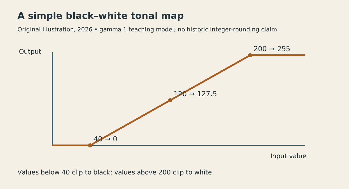
Original explanatory illustration, 2026. A gamma-one numerical teaching model, not a captured Levels interface or a reconstruction of its precise rounding.

This adjustment stretches an occupied middle range across the available output range. The difference between values near the middle becomes more pronounced. A scan with a narrow tonal range can look more forceful afterward.

The clipping is equally important. In our example, 20 and 40 both become zero. Values 200 and 230 both become 255. Differences have disappeared. The operation can improve the visual result while reducing information available for later adjustments.

A histogram helps the user see how many pixels occupy different value ranges. It doesn’t establish what those pixels depict or whether the darkest area should become completely black. The graph supplies evidence about distribution. It doesn’t provide an art director.

Select the scope before changing the values

An adjustment is often useful precisely because it applies to a chosen region. A sky and a foreground may need different treatment. A defect may need attention while neighboring texture should remain intact.

Photoshop’s 1990 guide documents selections, masks, and channels. It describes alpha channels for storing masks and distinguishes the image’s color channels from that additional selection information.³ Those facilities give an operation a scope more specific than “the whole picture.”

A mask can describe how strongly an operation applies at different positions. Conceptually, a fully selected position receives the adjustment, an unselected position doesn’t, and intermediate selection values permit a transition. This is a general explanation of masking, rather than a claim about a particular tool’s internal integer arithmetic.

The useful separation is between the image values and the decision about where to act. A stored selection can preserve the latter for reuse. It doesn’t preserve every edited object as an independently movable compositing layer. Giving an early feature a modern name can quietly turn it into a different feature.

Without modern layers, repeated work on the image made planning and saved copies particularly valuable. An author could make sophisticated changes, but the document didn’t offer today’s full collection of separate editable components. The technical capability and the convenience of revising it are different things.

Publishing supplied the destination

Thomas Knoll’s retrospective identifies publishing and graphic arts as important early markets. Digital-camera photography and convenient photographic printing were not yet the everyday workflow implied by today’s product name.¹

The original guide documents halftones, color separations, and conversion from RGB to CMYK for printed output.³ It is therefore misleading to summarize version 1 as having no CMYK relationship at all. Preparing an image for a printing process was part of the work.

This introduces another boundary between numbers and appearance. The monitor presents light. A printing process deposits ink. Different devices and media can produce different results from the data entrusted to them. Editing requires some understanding of the destination as well as the source.

Photoshop’s controls couldn’t make that whole chain effortless. They provided places where the decisions could be made: image dimensions, sample density, tonal range, selection scope, and output preparation. The application connected the stages without abolishing their differences.

What I find enduring in the first release is this combination of freedom and constraint. The image became editable numerical data. The available tools could change enormous numbers of values with very little physical effort. The user had to decide which information to preserve, which to discard, and how the result would eventually become visible.

The software made alteration easier. It also made it possible to inspect the decisions behind alteration. A good edit still begins with knowing what you’re trying to achieve before the pixels become obliging.

Footnotes

1. Russell Brady, Adobe interview with Thomas Knoll, February 18, 2015; anniversary introduction supplies February 19 1990 release date, creator interview supplies utility/application and early-market account. ↩ ↩² ↩³

2. Leonard Shustek, “Adobe Photoshop Source Code”, Computer History Museum, 2013; chronology, contributors, preserved 1.0.1 source, licensing and 1994 layers boundary. Its pictured splash screen is 1.0.7, not an exact launch artifact. ↩ ↩² ↩³ ↩⁴

3. Adobe, Photoshop User Guide, 1990, introduction pp.1–2 and opening-document discussion pp.7–8: channels, masks, printing and sample-resolution distinction. ↩ ↩² ↩³

4. Same 1990 guide, Chapter 14, pp.187 and205–206, distinct output-sizing and resampling operations. ↩

5. Same 1990 guide, Chapter 16, pp.286–289, input limits and gamma. Numerical dataset and formula above are original teaching examples; no historical runtime or exact integer-rounding claim. ↩